Random Forests for Complete Beginners
The definitive guide to Random Forests and Decision Trees.
| UPDATED
In my opinion, most Machine Learning tutorials aren’t beginner-friendly enough.
Last month, I wrote an introduction to Neural Networks for complete beginners. This post will adopt the same strategy, meaning it again assumes ZERO prior knowledge of machine learning. We’ll learn what Random Forests are and how they work from the ground up.
Ready? Let’s dive in.
1. Decision Trees 🌲
A Random Forest 🌲🌲🌲 is actually just a bunch of Decision Trees 🌲 bundled together (ohhhhh that’s why it’s called a forest). We need to talk about trees before we can get into forests.
Look at the following dataset:

If I told you that there was a new point with an coordinate of , what color do you think it’d be?
Blue, right?
You just evaluated a decision tree in your head:
That’s a simple decision tree with one decision node that tests . If the test passes (), we take the left branch and pick Blue. If the test fails (), we take the right branch and pick Green.

Decision Trees are often used to answer that kind of question: given a labelled dataset, how should we classify new samples?
Labelled: Our dataset is labelled because each point has a class (color): blue or green.
Classify: To classify a new datapoint is to assign a class (color) to it.
Here’s a dataset that has 3 classes now instead of 2:

Our old decision tree doesn’t work so well anymore. Given a new point ,
- If , we can still confidently classify it as green.
- If , we can’t immediately classify it as blue - it could be red, too.
We need to add another decision node to our decision tree:
Pretty simple, right? That’s the basic idea behind decision trees.
2. Training a Decision Tree
Let’s start training a decision tree! We’ll use the 3 class dataset again:

2.1 Training a Decision Tree: The Root Node
Our first task is to determine the root decision node in our tree. Which feature ( or ) will it test on, and what will the test threshold be? For example, the root node in our tree from earlier used the feature with a test threshold of :
Intuitively, we want a decision node that makes a “good” split, where “good” can be loosely defined as separating different classes as much as possible. The root node above makes a “good” split: all the greens are on the right, and no greens are on the left.
Thus, our goal is now to pick a root node that gives us the “best” split possible. But how do we quantify how good a split is? It’s complicated. I wrote an entire blog post about one way to do this using a metric called Gini Impurity. ← I recommend reading it right now before you continue - we’ll be using those concepts later in this post.
Welcome back!
Hopefully, you just read my Gini Impurity post. If you didn’t, here’s a very short TL;DR: We can use Gini Impurity to calculate a value called Gini Gain for any split. A better split has higher Gini Gain.
Back to the problem of determining our root decision node. Now that we have a way to evaluate splits, all we have to do to is find the best split possible! For the sake of simplicity, we’re just going to try every possible split and use the best one (the one with the highest Gini Gain). This is not the fastest way to find the best split, but it is the easiest to understand.
Trying every split means trying
- Every feature ( or ).
- All “unique” thresholds. We only need to try thresholds that produce different splits.
For example, here are the thresholds we might select if we wanted to use the coordinate:

Let’s do an example Gini Gain calculation for the split.
| Split | Left Branch | Right Branch |
|---|---|---|
First, we calculate the Gini Impurity of the whole dataset:
Then, we calculate the Gini Impurities of the two branches:
Finally, we calculate Gini Gain by subtracting the weighted branch impurities from the original impurity:
Confused about what just happened? I told you you should’ve read my Gini Impurity post. It’ll explain all of this Gini stuff.
We can calculate Gini Gain for every possible split in the same way:
| Split | Left Branch | Right Branch | Gini Gain |
|---|---|---|---|

After trying all thresholds for both and , we’ve found that the split has the highest Gini Gain, so we’ll make our root decision node use the feature with a threshold of . Here’s what we’ve got so far:
Making progress!
2.2: Training a Decision Tree: The Second Node
Time to make our second decision node. Let’s (arbitrarily) go to the left branch. We’re now only using the datapoints that would take the left branch (i.e. the datapoints satisfying ), specifically the 3 blues and 3 reds.
To build our second decision node, we just do the same thing! We try every possible split for the 6 datapoints we have and realize that is the best split. We make that into a decision node and now have this:
Our decision tree is almost done…
2.3 Training a Decision Tree: When to Stop?
Let’s keep it going and try to make a third decision node. We’ll use the right branch from the root node this time. The only datapoints in that branch are the 3 greens.
Again, we try all the possible splits, but they all
- Are equally good.
- Have a Gini Gain of 0 (the Gini Impurity was already 0 and can’t go any lower).
It doesn’t makes sense to add a decision node here because doing so wouldn’t improve our decision tree. Thus, we’ll make this node a leaf node and slap the Green label on it. This means that we’ll classify any datapoint that reaches this node as Green.
If we continue to the 2 remaining nodes, the same thing will happen: we’ll make the bottom left node our Blue leaf node, and we’ll make the bottom right node our Red leaf node. That brings us to the final result:
Once all possible branches in our decision tree end in leaf nodes, we’re done. We’ve trained a decision tree!
3. Random Forests 🌲🌳🌲🌳🌲
We’re finally ready to talk about Random Forests. Remember what I said earlier?
A Random Forest is actually just a bunch of Decision Trees bundled together.
That’s true, but is a bit of a simplification.
3.1 Bagging
Consider the following algorithm to train a bundle of decision trees given a dataset of points:
- Sample, with replacement, training examples from the dataset.
- Train a decision tree on the samples.
- Repeat times, for some .
To make a prediction using this model with trees, we aggregate the predictions from the individual decision trees and either
- Take the majority vote if our trees produce class labels (like colors).
- Take the average if our trees produce numerical values (e.g. when predicting temperature, price, etc).
This technique is called bagging, or bootstrap aggregating. The sampling with replacement we did is known as a bootstrap sample.

Bagged decision trees are very close to Random Forests - they’re just missing one thing…
3.2 Bagging → Random Forest
Bagged decision trees have only one parameter: , the number of trees.
Random Forests have a second parameter that controls how many features to try when finding the best split. Our simple dataset for this tutorial only had features ( and ), but most datasets will have far more (hundreds or thousands).
Suppose we had a dataset with features. Instead of trying all features every time we make a new decision node, we only try a subset of the features, usually of size or . We do this primarily to inject randomness that makes individual trees more unique and reduces correlation between trees, which improves the forest’s performance overall. This technique is sometimes referred to as feature bagging.
4. Now What?
That’s a beginner’s introduction to Random Forests! A quick recap of what we did:
- Introduced decision trees, the building blocks of Random Forests.
- Learned how to train decision trees by iteratively making the best split possible.
- Defined Gini Impurity, a metric used to quantify how “good” a split is.
- Saw that a random forest = a bunch of decision trees.
- Understood how bagging combines predictions from multiple trees.
- Learned that feature bagging is the difference between bagged decision trees and a random forest.
A few things you could do from here:
- Read about Information Gain, a metric similar to Gini Impurity that can also be used to quantify how “good” a split is.
- Experiment with scikit-learn’s DecisionTreeClassifier and RandomForestClassifier classes on real datasets.
- Try writing a simple Decision Tree or Random Forest implementation from scratch. I’m happy to give guidance or code review! Just tweet at me or email me.
- Read about Gradient Boosted Decision Trees and play with XGBoost, a powerful gradient boosting library.
- Read about ExtraTrees, an extension of Random Forests, or play with scikit-learn’s ExtraTreesClassifier class.
That concludes this tutorial. I like writing about Machine Learning (but also other topics), so subscribe if you want to get notified about new posts.
Thanks for reading!


